Dumbbell Calibration
Example 1
Calibration is the heart of the 3D-PTV. Therefore, having a better calibration will lead a better solution. There are two ways to calibrate the cameras. One can use traditional calibration (target block calibration) for which a three dimensional calibration target is required. The basic idea is to use a reference object with known coordinates. The calibration target should be seen by four cameras.
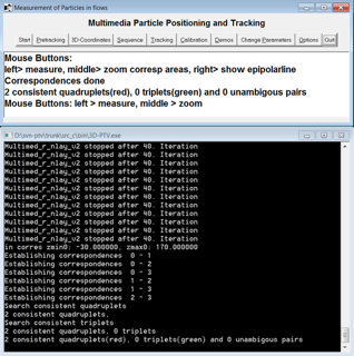
The other possibility is to use dumbbell calibration. In some applications, it is not feasible to use a calibration target inside or outside the investigation domain as a result of lack of space. The main idea is to move two points, with a fixed distance and known diameter, around the investigation domain. This movement will provide a 3D domain. As long as the points are seen by four cameras for all time instances, initial guesses converge. If the quality of the recordings is good enough, software will find two correspondences per image which are the points of dumbbell. Afterward calibration optimizes the distances by which the epipolar lines miss each other while maintaining the detected distance of the dumbbell points.
Here is an example of a dumbbell calibration:
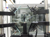
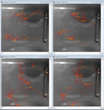
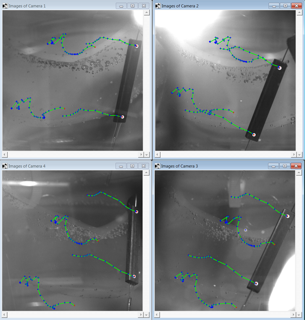
During the experiments, image splitter and four mirrors are used to mimic four virtual cameras. For a detailed preview, please check (http://ptv.origo.ethz.ch/wiki/four_view_image_splitter_3d_ptv). The investigation domain is the ascending aorta replica which has a diameter of 20 mm. The index of refraction is matched to avoid the noises.
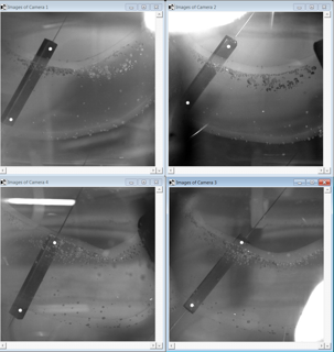
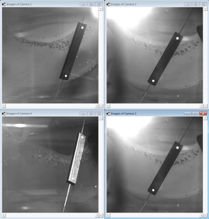
Firstly, dumbbell is moved behind the aorta. Then, it is moved in front of the aorta. All movements are recorded in 5000fps. The images are combined with a time step of 0.0176 s. It means that there are 62 time instances for dumbbell calibration.
The pre-calibration parameters and initial guesses are quite important to reach better results faster. For a rough initial guess, it will take some time to converge. The better initial guess, the less convergence time. Since it starts converging, the software will find two correspondences.
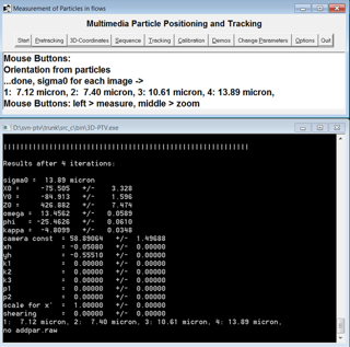
Dumbbell parameters will help to find the optimum eps values. One can start with a coarser numbers, then switch them into finer ones. After a certain number of iterations, the software converges. At this point, the quality of the result is related to user’s satisfactory. If the rms values are not good enough, one can go for a finer gradient descent factor and dumbbell penalty weight.
There is a small trick to go beyond converged numbers. One can apply shaking to the best initial guesses. Shaking improves the result. It helps to reduce error below 10 microns. But in any case one should back up ori files. Because sometimes it crashes!!!
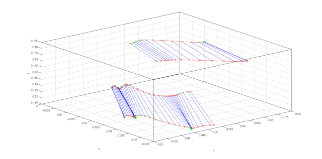
Now, you have a dynamic calibration by using dumbbell. Here are the plots of dumbbell tracking.
Example 2
Sometimes it is inconvenient to position a calibration target. Either because there is something in the way, or because it is cumbersome to get the entire target again out of the observation domain. It would be much easier to move a simple object randomly around the observation domain and from this perform the calibration.
This is what \ Dumbbell calibration\ is doing. The simple
object is a dumbbell with two points separated at a known distance. A
very rough initial guess is sufficient to solve the correspondence
problem for only two particles per image. In other words, the tolerable
epipolar band width is very large: large enough to also find the
correspondence for a very rough calibration, but small enough so as not
to mix up the two points. From there on, calibration optimizes the
distances by which the epipolar lines miss each other, while maintaining
the detected distance of the dumbbell points.
Unlike previous calibration approaches, Dumbbell calibration uses all camera views simultaneously.
Required input
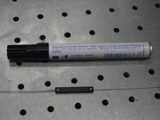
Somehow, an object with two well visible points has to be moved through the observation domain and recorder. The dumbbells points should be separated by roughly a third of the observation scale.
Note that the accuracy by which these dumbbell points can be determined in 2d, also defines the possible accuracy in 3d.
Processing:
Copy at least 500 images of the dumbbell (for each camera) as a tiff file to a new file Prepare target files using matlab code:
tau\_dumbbell\_detection\_db\_v3b. Every target file should contain only 2 points.Right click on the current run: choose main parameters.
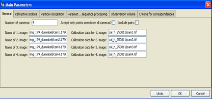
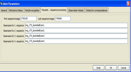
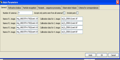
Main parameters:
write the name of the first dumbbell image, and the name of the calibration images you want to use.
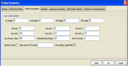
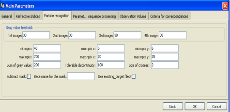
Particle recognition:
* since there are ready target files, mark \ use existing\_target\_files\.
Sequence processing:
Fill in the numbers of the first and last picture in the sequence processing, and the base name for every camera.
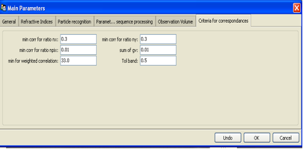
Criteria for correspondences:
min corr for ratio nx: min corr for ratio ny: min corr for ratio npix: sum of gv: min for weighted correlation: tol band: The number that defines the distance from the epipolar line to the possible candidate [mm].
Processing of a single time step:
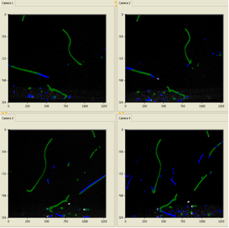
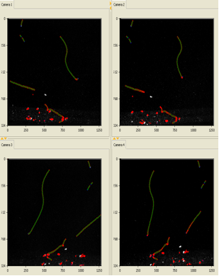
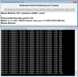
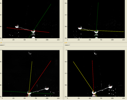
In the upper toolbar choose: start and then pre-tracking ,image coordinate, after that the two points of the dumbbell are detected. Then choose pre-tacking, correspondence. This establish correspondences between the detected dumbbell from one camera to all other cameras
you can press one point of the dumbbell in each camera and to see the epipolar lines.
The processing of a single time step is necessary to adjust parameters like grey value thresholds or tolerance to the epipolar line.
In the upper toolbar choose: sequence, sequence without display
In the upper toolbar choose: tracking, detected particles. Then tracking, tracking without display and then show trajectory.
Right click on the current run. choose calibration parameters:
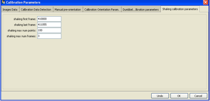
Dumbbell calibration parameters:
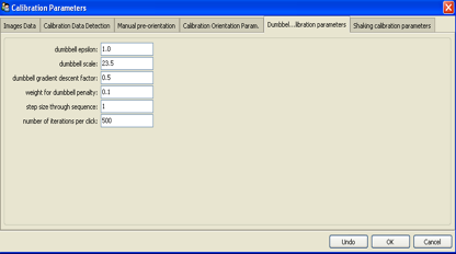
Eps [mm]: It is the tolerable bandwith by which epipolar lines are allowed to miss each other during calibration. should be the same number as the tol. band in Criteria for correspondences
Dumbbell scale [mm] :distance between the dumbbell points. It is quite important Since the algorithm optimizes two targets, the epipolar mismatch and the scale of the dumbbell particle pair
Gradient descent factor: if everything would be linear then a factor of 1 would converge after one step. Generally one is a bit instable though, so a more careful, but slow, value is 0.5.
Weight for dumbbell penalty: this is the relative weight that is given to the dumbbell scale penalty. with one it is equally bad to have dumbbell scale of only 24mm and to have epipolar mismatch of 1mm. After rough converge this value can be reduced to 0.01-0.2, since it is difficult to precisely even measure this scale.
Step size through sequence: it is step size. It could be different then 1 when the dumbbell recording is very long with successive images that are almost identical, then step size of 10 or so might be more appropriate.
In the upper toolbar choose : calibration and create calibration. choose orient with dumbbell.
See also: Dumbbell Calibration
Shaking calibration:
Processing of a single time step
Main parameters:
Write the name of the first image, and the name of the calibration images you want to use.
Particle recognition:
Don’t mark use existing_target_files. fill the particle recognition parameters in order to find the particles.
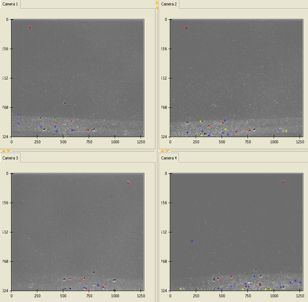
Press start in the upper toolbar. the four picture images from
main parameters, generalwill appear.
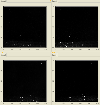
Under Pretracking the processing of a single time step regularly starts with the application of a highpass filtering (Highpass). After that the particles are detected (Image Coord) and the position of each particle is determined with a weighted grey value operator. The next step is to establish correspondences between the detected particles from one camera to all other cameras (Correspondences).
The processing of a single time step is necessary to adjust parameters like grey value thresholds or tolerance to the epipolar line.
Sequence:
After having optimized the parameters for a single time step the processing of the whole image sequence can be performed under Sequence .
Under main parameters, Sequence processing. Fill in the numbers of the first and last picture in the sequence processing, and the base name for every camera.
In the upper toolbar choose sequence with or without display of the currently processed image data. It is not advisable to use the display option when long image sequences are processed. The display of detected particle positions and the established links can be very time consuming.
For each time step the detected image coordinates and the 3D coordinates are written to files, which are later used as input data for the Tracking procedure.
Tracking:
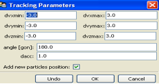
Tracking parameters:
Before the tracking can be performed several parameters defining the velocity, acceleration and direction divergence of the particles have to be set in the submenu Tracking Parameters. The flag‘
Add new particles position’ is essential to benefit from the capabilities of the
enhanced method. To derive a velocity field from the observed flow.
Tracking, Detected Particles displays the detected particles from the sequence processing.
Choose tracking, tracking without display. Again it is not advisable to use the display option if long sequences are processed. The tracking procedure allows bidirectional tracking.
Tracking, show Trajectories displays the reconstructed trajectories in all image display windows.