3D-PTV benchmark proposal
Introduction
During the meeting in Zurich in August 2009 the working group concluded that the three-dimensional particle tracking velocimetry (3D-PTV) is one of the established experimental approaches in the field of Particles in Turbulence. As a consequence, many algorithms, software packages have been developed over years by various research groups worldwide. This action is an attempt to learn best practices from each and to develop the open source particle tracking velocimetry that will combine the know-how of all the involved parties.
The first step, proposed during that meeting, was to develop few test cases that different research groups can use to test their own algorithms and software. The report of the groups will help to identify those performing best at different stages of the analysis and to expose the best practices to the other members of the action. There is a single important condition - open science. The codes, algorithms, data should be open to all the members of the action. The main goal is to make particle tracking better and accessible.
Test cases
At the moment there are few test cases available. These are of the two major types:
Synthetic images - for the demonstration purposes, we use the Standard PIV Images project. Specifically, we use the 3D standard images: http://www.piv.jp/image3d/image-e.html.
Experimental dataset
Synthetic images test cases
There are four cases on the Standard 3D Images website [1] that seem to fit our purpose of testing the tracking software packages:
Transient 3D flow field from 3 angles with wall refrection
Case 351 (Jet Shear flow)

+ Number of particles = 2000
        + Camera calibration Images are imX999.raw

(x,y,z) = (-0.8:0.0:0.8, -0.8:0.0:0.8, -0.8:0.0:0.8) 27 points

        + Three-cameras are on the holizontal plane

Case 352 (Jet Shear flow)

        + Number of particles = 300
        + Camera calibration Images are imX999.raw

(x,y,z) = (-0.8:0.0:0.8, -0.8:0.0:0.8, -0.8:0.0:0.8) 27 points

        + Three-cameras are on the holizontal plane

Transient 3D flow field from 3 angles with unknown wall refrection
Case 371 (Jet Shear flow)

        + Number of particles = 500
        + Camera calibration Images are imX999.raw

(x,y,z) = (-0.4:0.0:0.4, -0.4:0.0:0.4, -0.4:0.0:0.4) 27 points

        + camera parameters are not known

Case 377 (Jet Impinging flow)

        + Number of particles = 500
        + Camera calibration Images are imX999.raw

(x,y,z) = (-0.2:0.0:0.2, -0.2:0.0:0.2, -0.2:0.0:0.2) 125 points

        + cameras are set at the bottom of impinging plates
As we see, we can process the various cases and compare our algorithms versus the
given particle positions (aspects of stereo-matching, center-of-gravity, calibration and camera models, etc.)
given tracking (aspects of tracking, length of trajectory, filters along the trajectory, post-tracking “gluing” algorithms, etc.)
For example, comparing the case 352 and 371 will show if the effect of “known” vs “unknown” wall reflections on your camera model, comparing case 351 wit 352 will show the traceability parameter best, where the number of particles density is much higher in the “same” flow in case 351.
How to prepare and post the test case
For the demonstration purposes, we use the test case no 352: “Transient 3D flow field from 3 angles with wall refrection”. We find that the way Standard PIV Images project defined the test cases is simple and comprehensible. We suggest to adopt this way of formatting your experimental data for the test case. Below we report the way 3D-PTV software (ETH Zurich) is used to analyze the case #352 and to report the results for further analysis.
General description
1.Demo images- to provide a quick overview Source:
2.Textual information of the authors:
PIV Three-dimensional Standard Images #352
Generator: K. Okamoto (Univ. Tokyo) Program: ddr.c Date: March 27, 1998
3.Parameters:
Target Flow Field:  Jet impinging on the Wall
Reynolds Number:    3000
                     2cm
------------|   |------------
              |  15cm/s
              V
             XXX
             XXX
-----------------------------
Number of Particles inserted in the field       1000 Particles
Number of Particles visualized in one Image      320 Particles(average)
Diameter of Particles      5 pixel (average)
                           2       (standard deviation)
                           1       (minimum)
Maximum Velocity                 12 cm/s
Target Flow field                2cm x 2cm x 2cm
Time Interval between images     5 msec
Laser Illumination               Cylindrical from bottom (radius = 5cm) [almost whole illumination]
Water refractive index           1.33
Wall distance                    3 cm from center
orientation                 parallel to #1 camera image
Camera positions:
#0  Distance from center      20 cm
angle to X axis          -30 degree

#1  Distance from center      20 cm
angle to X axis            0 degree

#2  Distance from center      20 cm
angle to X axis           30 degree

No orientation variations were considered.
Sketch of the coordinate system:
                          ^ y
                           |
                           |/
               ------------+---------------> x
                          /|
                         / |
                        /
                       /z
                      L

TOP VIEW
                         |
                        O| Particles
           --------------+-----------------> x-axis
                        /|
                       / |
                      /  |        n=1.33(water)
           ==============|===================== WALL
                    /    |        n=1.00(air)
                   /theta|
                  / (-30)|(30)
                 /       |
               #0        |        #2 camera
            camera       |
                        #1 camera
                         |
                         | z-axis
                         V
Data description
Image Files (imX???.raw):
X:    camera# (0-2)
???:  serial# (000-144)   Total 720msec
Image size  256x256 pixel (8bit:256)

Calibration File (imX999.raw)
 Particles (Total 27 particles)
  x = -0.8, 0, 0.8 cm
  y = -0.8, 0, 0.8 cm
  z = -0.8, 0, 0.8 cm
Vector files(vec???.dat):
  x      y      z        u         v         w
-0.80  -0.80  -0.80   0.17542  -4.51977   0.01204
-0.80  -0.80  -0.60  -0.18245  -4.11870  -0.26516
-0.80  -0.80  -0.40  -0.78761  -3.38484  -0.41633

unit: x,y,z  [cm]
      u,v,w  [cm/s]
Particle Files(ptc???.dat):
#1 camera     #2 camera     #3 camera  intensity
ID    x      y      z      X      Y      X      Y      X      Y
4 -0.301  0.584  0.893 147.61  64.91  95.55  65.10  53.07  65.92 208.18
6 -0.898  1.266 -0.258   0.00   0.00   0.00   0.00  46.22   0.15 208.69
8  1.178  0.886  0.149 249.88  38.07 251.10  35.42 219.99  32.46 191.52
9  0.720 -1.242 -0.530 183.76 252.88 201.24 254.40   0.00   0.00 211.21

unit: x,y,z  [cm]
X,Y    [pixel]


The particle ID is unique number, therefore, the same particle could be easily tracked with checking the ID for serial particle files.
Thanks to the authors of the Standard 3D PIV Images: Dr. Okamoto (okamoto@tokai.t.u-tokyo.ac.jp)
PIV Standard Images test case 352
We keep a mirror copy of the data for the case 352 on case 352 copy
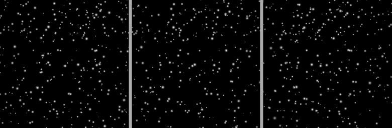
Synthetic data were used to validate the algorithm. The synthetic data were from the PIV-STD library that was developed by the Visualization Society of Japan and served as the benchmark for many PIV/PTV research efforts (Okamoto et al 2000, Ruhnau et al 2005, Kim and Sung 2006). Data set 352 was chosen, which describes a jet flow impinging on a wall. The flow is transient and three dimensional. Data from Camera 0, frame 0–89 were adopted. At each frame, about 300 particles were in the observed region, which has a size of 256 by 256 pixels. The fluid motion was captured by three cameras. The particle spacing displacement ratio (PSDR), which is defined as the ratio of the average particle spacing to the mean particle displacement between two consecutive frames and serves as an important indicator to the difficulty of the tracking process (Malik et al 1993), is about 3.4 for thewhole image domain. However, compared to the left half of the images, the right half contained denser particles and larger particle displacement (see figures 4 and 5), which results in a lower PSDR. The PSDR is about 2.6 for the right half of the image domain and about 2.2 for the right quarter of the image domain. Such a small value makes it hard to track particles through 90 frames (Malik et al 1993).
** A multi-frame particle tracking algorithm robust against input noise**, by Dongning Li, Yuanhui Zhang, Yigang Sun andWei Yan, Meas. Sci. Technol. 19 (2008) 105401
3D-PTV software applied to the test case #352 (Standard PIV Images project)
Here we report the technical procedures, the results and the analysis of the case #352 processed using 3D-PTV software (ETH Zurich, Tel Aviv University).
Download images and the data for the test case #352 from the original web site http://piv.vsj.or.jp/piv/image3d/image352.html (just in case the website/data will disappear, we’ll keep a local copy on our web server)
Obtain 3D-PTV software from the website: http://www.openptv.net/docs/ (for Windows platforms, if no source is needed, the ZIP file below includes the executable, so it’s plug-n-play ready test case)
Pre-processing procedure
Download the ZIP file with the directory ready for use with the software. Extract the file into the experiment directory, e.g. C:/PTV/test352
verify it has the directory structure:
C:/PTV/test352
                /img
                /res
                /cal
                /parameters
read more about the software handling on http://www.openptv.net/docs/add_doc.html
convert RAW images to TIFF images (no compression, 8 bit). On Windows , IrfanView (with plugins) used for batch image conversion and rename.
image0XXX.raw -> cam1.1XXX (1XXX= 1000 to 1144). Note that we also name our cameras: 1,2,3 as the PIV STD project calls them 0,1,2
move the images into the the sub-directory /img
We already converted the calibration images: im0999.raw -> cam1.tif, im1999.raw -> cam2.tif, im2999.raw -> cam3.tif
and added the calibration images to the sub-directory /cal
Basically, we convert the information provided for this test case into the calibration files, compatible with the 3D-PTV software. The camera configuration is well explained on the Evaluation of standard PIV images website by Georges Quenot from http://www-clips.imag.fr/mrim/georges.quenot/vsj-eval/evaluation3.html
This is precisely the same coordinate system as used by the 3D-PTV software. Therefore the conversion of the parameters is easy:
in the /cal directory you’ll find the *.ORI files for each camera. These consist of
 101.8263 -9.9019 65.1747 projective center X,Y,Z, [mm]
 0.4151383 -0.0069793 1.5073263 omega, phi, kappa [rad]
 0.0634259 -0.9979621 -0.0069792 rotation matrix (3x3)
 0.9130395 0.0608491 -0.4033067 [no unit]
 0.4029095 0.0192078 0.9150383
 -0.6139 -0.0622 xp, yp [mm]
 8.7308 principle distance [mm]
 0.0 0.0 30.0 window (glass) location [mm]
 so the three cameras are oriented approximately:

 cam1.tif.ori
 -100.3781      0.0117    173.0085
 0.0000154  -0.5432731  -0.0000624
 0.8560213  0.0000534 -0.5169406
-0.0000704  1.0000000 -0.0000132
 0.5169406  0.0000477  0.8560213
 0.0000   0.0000
 20.0000
 0.000000000000000    0.000000000000000    30.000000000000000

 cam2.tif.ori
 0.4331     -0.0829    199.4893
 0.0005046   0.0022530   0.0001731
 0.9999974 -0.0001731  0.0022530
 0.0001743  0.9999999 -0.0005046
-0.0022529  0.0005050  0.9999973
 0.0000   0.0000
 20.0000
 0.000000000000000    0.000000000000000    30.000000000000000

 cam3.tif.ori
 101.0432      0.0872    172.5569
 -0.0004084   0.5476053   0.0000590
 0.8537737 -0.0000503  0.5206442
 -0.0001537  0.9999999  0.0003487
 -0.5206442 -0.0003777  0.8537737
 0.0000   0.0000
 20.0000
 0.000000000000000    0.000000000000000    30.000000000000000

 Calibration File (imX999.raw)
 Particles (Total 27 particles)
 x = -0.8, 0, 0.8 cm
 y = -0.8, 0, 0.8 cm
 z = -0.8, 0, 0.8 cm
 is converted into a text file in the format, compatible with the 3D-PTV software - four columns of: ID, X, Y, Z, using the Matlab code (attached to the ZIP file):
    1    -8    -8    -8
    2    -8     0    -8
    3    -8     8    -8
    4     0    -8    -8
    5     0     0    -8
    6     0     8    -8
    7     8    -8    -8
    8     8     0    -8
    9     8     8    -8
   10    -8    -8     0
   11    -8     0     0
   12    -8     8     0
   13     0    -8     0
   14     0     0     0
   15     0     8     0
   16     8    -8     0
   17     8     0     0
   18     8     8     0
   19    -8    -8     8
   20    -8     0     8
   21    -8     8     8
   22     0    -8     8
   23     0     0     8
   24     0     8     8
   25     8    -8     8
   26     8     0     8
   27     8     8     8
 Processing (particle locations, stereo-matching, 3D positions, tracking) is then according to the standard 3D-PTV procedure. All the parameters are given in the ZIP file and reproduced here as a snapshot of the respective menus:
 Following 3D-PTV tutorials we proceed with:
 Start -> Tracking -> Sequence/Tracking to complete the full cycle of processing. The results appear in two subdirectories:

 2D particle locations in pixels, per camera in /img directory, named cam?.1XXX_targets
 3D particle locations and tracking information in /res directory named ptv_is.1XXX
Comparsion of results
Test case 371
Here we first copy the original description of the experimental conditions from their case 377 website:
No.      377    Unit
Image Size      256 x 256       pixel
Area    1 x 1   cm
Laser Illumination      Volume  mm
Interval        0.001   sec
Max. Velocity   10      pixel/interval
Max. out-of-plane Velocity      ??      %
DATA DOWNLOAD

* The format of the images are RAW data.[64KB]
* The particle data file[100KB] contains; (1) particle ID, (2-4) particle 3d location [x,y,z] (cm),
(5,6) particle location in Image 0 [X,Y] and (7,8) particle location in Image 1 [X,Y] and
(9,10) particle location in Image 2 [X,Y] and (11) maximum intensity of the particle [I].
The particle ID is unique, so that the same particle location could be correctly tracked with using
the serial particle files. Please see the example
* The vector file[50KB] contains; (1-3) node of the image (X,Y,Z) [cm] and (4-6)
vector (U,V,W) in the unit of [cm/s] Please see the example


PIV Three-dimensional Standard Images    #377


Generator:  K. Okamoto  (Univ. Tokyo)
Program:    ddr.c
Date:       March 27, 1998


Parameters:
 Target Flow Field:  Jet impinging on the Wall
 Reynolds Number:    3000

                      2cm
         ------------|   |------------
                       |  15cm/s
                       V


                    XXX
                    XXX
         -----------------------------

 Number of Particles inserted in the field      40000 Particles
 Number of Particles visualized in one Image      500 Particles (average)

 Diameter of Particles      5 pixel (average)
                            2       (standard deviation)
                            1       (minimum)

 Maximum Velocity                 12 cm/s
 Target Flow field                5mm x 5mm x 5mm
 Time Interval between images     1 msec

 Laser Illumination               Cylindrical from bottom (radius = 1cm)

 Water refractive index           1.33
 Wall distance                    7 mm from center
      orientation                 y-direction  (simulate impinging plate)

 Camera positions
    #0  (x,y,z) = (5.77, -10, 0)

    #1  (x,y,z) = (-2.88, -10, -5)

    #2  (x,y,z) = (-2.88, -10, 5)


  Small Orientation variations were considered.


                                    ^ y
                                    |
                                    |/
                        ------------+---------------> x
                              #2   /|
                                  / |      #1
                          #3     /
                                /z
                               L


           Side View              ^
                             Jet  | y-axis
                                  |
                                 O| Particles
                    --------------+-----------------> x-axis
                                 /|        n=1.33(water)
                    ==============|2mm==================
                               /  |        n=1.33(acryl)
                    ==============|7mm================== WALL
                             /    |        n=1.00(air)
                            /     |
                           /      |
                          /       |
                        #2,3      |        #0 camera
                     camera       |
                                  |

            The wall surface is (y=-7mm)
            Jet impinging plate is (y=-2mm)
            Visualized region is (-2,-2,-2) < (x,y,z) < (2,2,2)mm


Image Files (imX???.raw)

  X:    camera# (0-2)
  ???:  serial# (000-200)   Total 200msec

  Image size  256x256 pixel (8bit:256)


 Calibration File (imX999.raw)
   Particles (Total 125 particles)
     x = -0.2, -0.1, 0, 0.1, 0.2 cm
     y = -0.2, -0.1, 0, 0.1, 0.2 cm
     z = -0.2, -0.1, 0, 0.1, 0.2 cm


Vector files  (vec???.dat)

   x      y      z        u         v         w
 -0.80  -0.80  -0.80   0.17542  -4.51977   0.01204
 -0.80  -0.80  -0.60  -0.18245  -4.11870  -0.26516
 -0.80  -0.80  -0.40  -0.78761  -3.38484  -0.41633

   unit: x,y,z  [cm]
         u,v,w  [cm/s]


Particle Files  (ptc???.dat)
                             #1 camera     #2 camera     #3 camera  intensity
   ID    x      y      z      X      Y      X      Y      X      Y
    4 -0.301  0.584  0.893 147.61  64.91  95.55  65.10  53.07  65.92 208.18
    6 -0.898  1.266 -0.258   0.00   0.00   0.00   0.00  46.22   0.15 208.69
    8  1.178  0.886  0.149 249.88  38.07 251.10  35.42 219.99  32.46 191.52
    9  0.720 -1.242 -0.530 183.76 252.88 201.24 254.40   0.00   0.00 211.21

   unit: x,y,z  [cm]
         X,Y    [pixel]

   The particle ID is unique number, therefore, the same particle could
   be easily tracked with checking the ID for serial particle files.


If you have any questions, please contact Dr. Okamoto
(okamoto@tokai.t.u-tokyo.ac.jp)
Download and prepare the test case
1.Download the images, point and vec files from the original website using [2] . 2.Create 3D-PTV directory:
C:/PTV/case377
                /img
                /res
                /cal
                /parameters
Convert RAW images into TIFF (8 bit) images using IrfanView (on Windows), ImageMagick or Matlab. The name convention is cam1.XXX cam2.XXX cam3.XXX (not .tif extension)
Use the attached [3] Matlab file (remove .txt extension) to generate the calibration images and necessary ASCII files (see >> help ptc999_to_man_ori_377 for more information).
5.The orientation of the cameras turned to be quite tricky as the authors didn’t mention the rotation around the imaging axis. Never mind, the ORI files are attached (remove .txt extension) . These could be significantly improved using iterative SHAKING algorithm of Beat.
Sample run
If all the previous steps were successful, then running start.bat will open the main window. From there, Start, then Tracking -> Sequence/Tracking will be the fastest way of checking it. At the end, Tracking -> Show trajectories should show something of the kind:
Prepare calibration
function ptc999_to_man_ori_377(dir1,dir2,midplane)
% PTC999_TO_MAN_ORI_377(DIRNAME1,DIRNAME2,MIDPLANE)
% takes the PTC999.DAT file from DIRNAME1 as an input
% and generates all the necessary files for the 3D-PTV software
% (almost) automatic calibration in DIRNAME2:
% MAN_ORI.DAT
% MAN_ORI.PAR in /parameters
% CAL377.TXT
% CAM1.TIF, CAM2.TIF, CAM3.TIF in /cal
%
% There is only CAM1-3.TIF.ORI files are missing.
%
% MIDPLANE = 0 or 1 (false or true) - useful if only the midplane
% points are used for the calibration.
%
% Author: Alex Liberzon
%

if ~nargin
    dir1 = 'c:\PTV\benchmarks\piv_std_377\ptc\';
    dir2 = 'c:\PTV\Software\sortgrid_from_initial_guess_Oct09\case377\';
    midplane = 0;
end
% PTC999_TO_MAN_ORI_377

% read ptc999.dat file from the case 377
d = load(fullfile(dir1,'ptc999.dat'));

cal = fullfile(dir2,'cal377mid.txt');
dat = fullfile(dir2,'man_ori.dat');
par = fullfile(dir2,'parameters','man_ori.par');
cam1 = fullfile(dir2,'cal','cam1.tif');
cam2 = fullfile(dir2,'cal','cam2.tif');
cam3 = fullfile(dir2,'cal','cam3.tif');

% cm -> mm
d(:,2:4) = d(:,2:4)*10;

% transform axis: x->x y->-z z -> y
tmp = d;
d(:,3) = tmp(:,4);
d(:,4) = -tmp(:,3);

% indices:
% d(:,1) = d(:,1) + 1;

% if one plane only:
if midplane
midplane = find(d(:,4) == 0);
d = d(midplane,:);
d(:,1) = 1:size(d,1);
id = [1,5,21,25];
else
    d(:,1) = d(:,1) + 1;
    id = [1,5,121,125];
end


% write cal377.txt
fid = fopen(cal,'w');
fprintf(fid,'%5d %9.4f %9.4f %9.4f\n',d(:,1:4)');
fclose(fid);

% choose points
id = [1,5,21,25];
fidpar = fopen(par,'w');
fiddat = fopen(dat,'w');
for i = 1:4
    fprintf(fidpar,'%3d\n',d(id,1));
end
for i = 1:4
    fprintf(fiddat,'%6.3f %6.3f\n',d(id(i),5:6));
end
for i=1:4
    fprintf(fiddat,'%6.3f %6.3f\n',d(id(i),7:8));
end
for i=1:4
    fprintf(fiddat,'%6.3f %6.3f\n',d(id(i),9:10));
end

fclose(fidpar);
fclose(fiddat);

% generate images:
% Image generation parameters
Radius = 2;
sx = 256;
sy = 256;

%% Cam1
x = d(:,5);
y = d(:,6);
% figure, scatter(x,y)
bw = uint8(zeros(sx,sy));
for j = 1:length(x)
    output_coord = plot_circle(x(j),y(j),Radius);
    bw = imadd(bw,uint8(poly2mask(output_coord(:,1),output_coord(:,2),sx,sy)));
end
bw(bw>0) = 255;
% figure, imshow(bw)
imwrite(bw,cam1,'tiff','compression','none')

%% Cam1
x = d(:,7);
y = d(:,8);
% figure, scatter(x,y)
bw = uint8(zeros(sx,sy));
for j = 1:length(x)
    output_coord = plot_circle(x(j),y(j),Radius);
    bw = imadd(bw,uint8(poly2mask(output_coord(:,1),output_coord(:,2),sx,sy)));
end
bw(bw>0) = 255;
% figure, imshow(bw)
imwrite(bw,cam2,'tiff','compression','none')

%% Cam1
x = d(:,9);
y = d(:,10);
% figure, scatter(x,y)
bw = uint8(zeros(sx,sy));
for j = 1:length(x)
    output_coord = plot_circle(x(j),y(j),Radius);
    bw = imadd(bw,uint8(poly2mask(output_coord(:,1),output_coord(:,2),sx,sy)));
end
bw(bw>0) = 255;
% figure, imshow(bw)
imwrite(bw,cam3,'tiff','compression','none')
Attachment
Experimental dataset
Test case from Wesleyan University
The data is posted on http://gvoth.web.wesleyan.edu/PTV/Wes_data.htm
After some transformations (the detailed instructions will be posted soon), Alex got this:
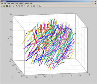
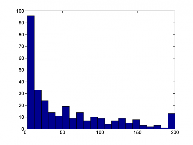
There are 310 trajectories of various length, few longest are 200 frames (full run) long:
some e-mail that should be converted into the website
1.The data is Wesleyan data. 2.The software is 3D-PTV software, v1.02 (I installed the batteries-included-version http://ptv.origo.ethz.ch/wiki/Windows_Installer_Package) 3.All the changes were performed in the /test subfolder of this installation in order to be sure that the same parameters are set up. (parameters.zip is attached).
- our coordinate system is different and it’s not flexible, so I had to change it to:
x -> z, y -> x, z -> y
renamed image files to the format of cam1.10001 - cam4.10200(I added 10000 for the convenience, I never sure about 0xxx format of the extension)
- renamed calibration images
av_calib1_edit -> cam1.tif
We use ‘negative’ images, i.e. white dots on dark background. some matlab trick is attached
 our coordinate system is different and it's not flexible, so I had to change it to:
    x -> z, y -> x, z -> y
renamed image files to the format of  cam1.10001 - cam4.10200(I added 10000 for the convenience, I never sure about 0xxx format of the extension)
renamed calibration images
    av_calib1_edit -> cam1.tif
We use 'negative' images, i.e. white dots on dark background. some matlab trick is attached
created orientation files. first version was simply the copy of the information from Wes_data.htm, e.g. for camera 1:
650.0 70.0 650.0 <-- x,y,z camera position
0.2 0.0 0.0      <-- angles, 0.2 rad looking d
0 1 0
0 0 1

0.0 0.0       &nownwards
1 0 0
bsp; <--- xp,yp, default
100.0           <--- focal distance, unknown parameter
500.0 0.0001 500.0 <--- interface, perpendicular to the camera, radius of the tank
the attached *.ori files are already after static (using the calibration plate) and dynamic calibration (shaking).
created calblock.txt file that numbers the points on the calibration plate from 1 to 100, such that:
1 ... 9
.......
91 .. 100
top left is 1 and top right is 9, bottom left is 91 and bottom right is 100. the origin is point 95.
changed the Main Parameters to have 10 mm glass and images of the 1280 x 1024 pixels. I didn’t know the pixel size, changed it to 10 micron (should not be a big problem on average) and I do not know how much it affects the final results.
using manual tagging of points 1,9,91,100 and few iterations, the data was pretty well calibrated, due to large distance from the calibration plane, the numbers are below 1 micron accuracy.
added dynamic calibration using first 50 frames. the parameters folder is zipped and attached.
standard run of the 3D-PTV software (v1.02, from the standalone installation, see origo) with sequence/tracking and tracking backwards created the data which is attached in wes_data.zip. The files were converted from _targets files to the cam1,2,3,4_2D.dat using our Matlab subroutine (attached, et_targets_to_bench2D_format).
the branch of our post_processing software (see on origo) that is called bench_3D_output creates the text file (inside the wes_data.zip) called wes_bench3d.txt. the format is as it was before: x,y,z,frameId,trajID
Hopefully, everyone can now re-run it with the same settings to get the same/close result. If possible, someone has to repeat the steps (now it’s easier) and type a tutorial of how to use Wesleyan data in 3D-PTV software. Since it’s a nice one-plane calibration that evolves as a dynamic calibration is added - we could consider this case as a nice tutorial for the 3D-PTV users. we can also test various dynamic calibrator algorithms on this case, as a part of the post-benchmark collaboration.